
A Model Hedge
Analyzing a portfolio containing equities and non-linear securities (such as options) typically requires both a factor model and Monte Carlo simulation. Axioma Risk delivers the best of both worlds — simulation with full repricing and factor model risk decompositions.
The Challenge
An equity portfolio will often be analyzed or even constructed with the aid of a factor model. The bets and risks will to some degree be understood in the language of factors. For example, a manager may choose to be overweight Value, or neutralize some particular industry. If the portfolio contains non-linear securities (such as a put option, perhaps acting as a hedge) then one must deal with a number of additional effects. First, the non-linear security will usually introduce an asymmetry between positive and negative returns. A large positive equity return may have little effect on a put, for example, but a large negative return may significantly increase its value. These non-linear effects are not captured by a model that assumes all securities are linear. This usually requires a Monte Carlo simulation with full repricing to get accurate risk numbers. Second, non-linear assets will be exposed to risk factors not typically found in equity factor models. For example, an option will be exposed to interest rates and implied volatility. Finally, assets such as options will age. For example, an option that expires in two months, during the course of a one-month risk horizon, becomes a one-month option, at which point its risk characteristics and price are quite different from those on the analysis date.
The Solution
Axioma Risk addresses all the above issues.
- First, there is no tension between using a factor model and simulation. We directly simulate the factor model, allowing risk reports that decompose risk along familiar factor lines. We also incorporate various nuances of a well-estimated factor model, such as different decay factors for volatility, correlation, and specific risks, as well as the use of Newey-West estimators. In fact, what one simulates can be chosen by the user. For example, in effect what we have just described is mapping equities to a factor model, but other choices are possible. For instance, a user could map equities to a dense model (where each asset is a separate risk factor), albeit at the cost of losing the factor decomposition of risk.
- Second, any additional risk factors are simulated (with correct correlations) along with the factors from the risk model. In the case of an option, this would result in the simulation of several nodes from an interest-rate curve, as well an implied volatility factor.
- Finally we come to aging. This can be tackled in at least two ways. The first is to skirt the issue. If one were computing risk over a one month horizon, one might use the predicted distribution of market returns corresponding to that horizon, but assume (counterfactually) that the returns are realized instantaneously, thus obviating the need for any aging whatsoever. While simple, this approach suffers from the drawback that the risk profile of any derivatives in the portfolio may have changed by the time they reach the end of the risk horizon, and thus the risk analysis will be biased. Alternatively, one may address the issue head-on and age all securities appropriately. Thus during risk computations an option will be priced according to its time-to-expiry at the end of the risk horizon, rather at its start. This is what one would expect since we are computing a risk measure for the end of the risk horizon (rather than its start). One minor wrinkle in this computation is what to use as the security’s reference value. This is needed when computing Value-at-Risk, since one needs to compute losses as the difference between the reference value and a simulated value. For the instantaneous aging (namely, no aging) this is trivial — it is the value of the security on the analysis date. For proper aging we must age the security (and if appropriate, the market) and value it accordingly; this could be summarized as use the modal rather than the mean price.
An Example
In this section we illustrate the above ideas with a simple example. We start with an equity-only portfolio, in this case the constituents of the S&P 500. A more interesting example might be an optimized portfolio, perhaps with a benchmark; but we will keep things simple. Our goal will be to hedge away a certain risk. In the interest of simplicity we will try to hedge away our exposure to Apple by adding a put option to the portfolio. Again, one can imagine a more complex scenario. For example, hedging away unwanted factor risk by adding a collection of options — certainly more interesting, but at the cost of lengthening the exposition.
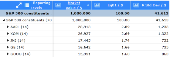
Figure 1
Figure 1 shows the larger constituents of the S&P 500 (as of the beginning of last August). Since Apple has the largest weight, we will choose to hedge out exposure to it using a put, and then analyze the resulting risks. The same figure shows the risk of each component of the index. These were computed using a linear methodology and we refer to them as parametric risks or parametric standard deviation (hence the prefix “P” in column heading “P Std Dev”). In general, all statistics computed using a linear non-simulation methodology will receive a prefix of “P” in this document. In addition, the parametric computations will be computed using the instantaneous aging methodology.
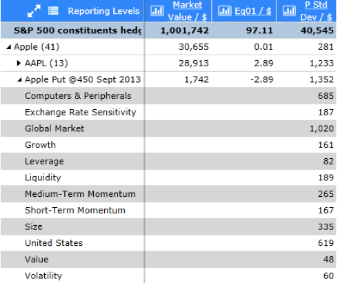
Figure 2
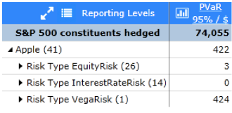
Figure 3
Next we hedge, in this case with a slightly out-of-the-money put on Apple, expiring about a month and half from the analysis date. We size it so it delta-hedges the equity position on the analysis date (see the Eq01 column in Figure 2). Note also in Figure 2 that we can see a full risk decomposition of our option along factor model dimensions (each line being the standalone VaR for that source of risk). Note that so far everything is linear. In fact, the linearity (as well as the absence of aging) can be seen clearly in Figure 3, where rearranging the risk decomposition to show first Apple (and its option) and then risk type shows almost all equity risk to have been hedged out (as expected since we delta hedged). Although the analysis is linear, we already pick up vega risk (as well as a very small amount of interest rate risk).
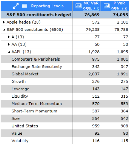
Figure 4
Given the presence of an option in our portfolio, we now generate reports with VaR computed using Monte Carlo simulation (with full repricing for the option). Our Monte Carlo computations will also use full aging (in contrast to the parametric computations). In Figure 4 we see this comparison, with Monte Carlo VaR labeled “MC 95% VaR”. First note that for the sub-portfolio labeled “S&P 500 constituents” the linear and Monte Carlo computations agree closely. This is expected since this sup-portfolio is composed of linear securities (equities) and hence the discrepancy is caused by simulation noise. The sub-portfolio labeled “Apple hedge” contains just the option and here there is a large difference between the linear and the non-linear computation, as expected. In fact, the non-linear VaR is less than the parametric VaR since an out-of-the-money put cannot lose a great deal of value. In this Figure we can also see that although we are simulating, we still have access to the usual factor decomposition (for both equities as well as for derivatives).
An interesting effect appears after adding the hedge (see Figure 5): the MC VaR of the subset consisting of Apple and its hedge is less than the parametric VaR. Figure 6 shows that this can be attributed to vega risk. On reflection this is expected since this risk is unhedged (in fact it was introduced by the hedge) and the option has limited downside when implied vols move (see Figure 7), a fact the linearized computation is unable to capture.
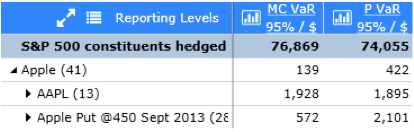
Figure 5
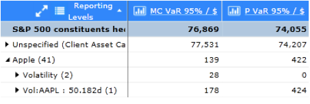
Figure 6
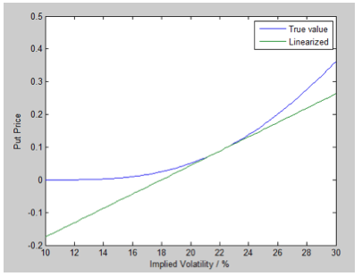
Figure 7
Conclusion
This document discussed how linear factor models can happily coexist with non-linear pricing and Monte Carlo simulation. One final comment worth making is that, while we have focused on equities, the ideas are very general, and perhaps certain aspects (such as aging) are more central to other asset classes. Within the framework discussed above, one can analyze fixed income, FX, and commodities. The analyses can be linear, Monte Carlo, or historical, but always consistent with each other.